Final Post

Introduction

This project aims to explore the research done on automatic abstract text summarization and look for ways to improve the model. The topic of automatic text summarization was chosen because of my interest in cutting down time spent on reading materials that could be dry and dull on occasions. With the rise of popularity in Neural Networks and my previous knowledge in Machine Learning, I wanted to study and learn more about the development of automatic text summarization tools. While there are two fields of automatic text summarization (extractive and abstractive), I focus on abstractive approaches due to its higher difficulty and significance in creating a human-like summarization tool. Here is a general overview:

Existing Work

Automatic text summarization is considered a sequence-to-sequence problem (seq2seq); meaning, it's a prediction problem that takes a sequence as input and requires a sequence as output. For seq2seq problems, Recurrent Neural Networks (RNN) have been used because of it specialization in forming connections between units to form a directed graph along a sequence to retain learned information throughout the process. Although RNN has proven its strength in seq2seq problems, because the network applies the same weight to learned information throughout the learning process, it tends to either vanish information that wasn't considered important in the beginning or explode information that was deemed important in the beginning. Because this choice made in the beginning is not always correct, this vanishing/exploding gradient problem can mislead the model by a mile. 

To adjust for this problem, Long-Short Term Memory (LSTM) models have been developed where this model adds a cell-state that runs straight down the chain with regulated gates that add/remove information from the network. While having this pipeline of data that runs throughout the network to retain/remove important information, there are still many problems that need to be solved, two of which are outputting repeated sentences/information and dealing with out-of-vocabulary (OOV) tags.

Baseline Model

In order to solve these two problems, researchers from Google and Stanford created Pointer-Generator Networks (PGN). PGN utilizes two notable features: pointers and coverage mechanism. Here is a diagram of the baseline mode:

There are two inputs: the source text and the reference summary written by a human for the source text. The model takes the source text and runs each word w_i through a single-layer bidirectional LSTM encoder. This then becomes the encoder hidden states h_i. On the other hand, the reference summary is put through a single-layer unidirectional LSTM decoder one word at a given time t and produces the decoder hidden states s_t. On a side note, reference summary is used for the decoder during training while the previous word emitted by the decoder is used during testing. Using both h_i and s_t, the attention distribution a^t is created with the following equations:

where v, W_h, W_s, and, b_attn are learnable parameters. Attention distribution is a probability distribution over the srouce words that tells the decoder where to look to produce the next word; in other words, where the attention should be at.

Here the coverage mechanism kicks in with the coverage vector. The coverage vector c^t is a distribution over the source document words that represents the degree of coverage that those words have received from the attention mechanism so far. 

Because this vector keeps track of how much each word has received attention, it can detect when a word has been covered before. This prevents the words/information from being outputted again so that no repeated information is produced in the generated summary; thus, solving the problem of repeated information.

The context vector h^*_t is then created from the following:

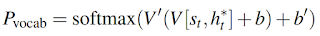
This is the representation of what has been read from the source for this step t. Context vector, along with decode hidden states, is then used to create the vocabulary distribution P_vocab. 

This is the probability distribution over all of the words in the given vocabulary pool. The word with the highest probability is the word that is most likely to be outputted from the vocabulary pool in creating the generated summary.

So now we have two places to look at when figuring out which word to output: the attention distribution and the vocabulary distribution. This is where the solution to dealing with OOV tags comes in. For most of the models out there, if it encounters a word that is OOV, it would instead output <UNK> tag. For example, let's say the model has decided that it's going to generate the word Manchester. While this word may be important, it is very possible for the word to not be in the vocabulary pool. Because Manchester cannot be found in the vocabulary pool, the model would then produce <UNK> creating the summary: There was a robbery in the city of <UNK>. This is rather an awkward summary and leaves out important information. To address this issue, PGN utilizes generation probability p_gen.

where x_t is the decoder input and vectors w_h^*, w_s, w_x, and scalar b_ptr are learnable parameters. p_gen is then used to create the final distribution P(w).

This is basically a soft switch to choose between generating a word from the vocabulary pool or copying a word from the input sequence by sampling from the attention distribution. If the model detects that an OOV is to be outputted, it switches towards the attention distribution in creating not an unknown tag but rather the word itself straight from the source document. Hence, dealing with the problem of creating a confusing summary with unknown tags.

While PGN solves the problems of repeated information and unknown tags, it still has a problem: pronoun ambiguity.

Problem with Pronouns

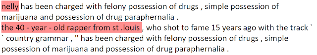
The baseline model struggles at times with pronouns in ways where it produces pronouns in generated summaries without defining the pronoun first and outputting pronouns where it is ambiguous as to which noun the pronoun is referring to. For example, here is a reference summary:

And here is a summary generated by the baseline model:

From comparing these two summaries, one can notice that the generate summary is a lot longer and contains information that might be considered too much. But it is important to note that the important information are all there. Therefore, while it this generated summary can be seen as a good summary, it fails to define the pronoun rapper before defining it as nelly. If the reader is unfamiliar with the rapper Nelly and is unfamiliar with the whole rapper scene in general, it could be very confusing who the rapper from st.louis is and where the word nelly came from in the middle of the summary. In order to counter this problem, I came up with two solutions.

Two Models

This model primarily focuses on pre-processing and post-processing the data to deal with the pronoun ambiguity. A lot of research and work has been put into the field of coreference resolution where people have looked for ways to solve pronoun ambiguity. From this field, I found a Coreference Resolution Model using spaCy that has a feature that detects pronouns and the nouns that the pronouns are referring to. Using this model and the baseline model, I created the following:

Here I take the reference summaries and before they are put through the single-layer unidirectional LSTM decoder, I run them through the Coreference Resolution Model to detect the pronouns and the nouns they are referring to. I then save the obtained information into a dictionary format to a local storage (e.g. {Wayne: [he, his, him, student]}). After saving the information, I replace all the pronouns with the nouns they are referring to (e.g. The text "Wayne saw himself." becomes "Wayne saw Wayne."). By doing so, when the baseline model looks to the reference summary to see what it's supposed to be outputting, there should be no pronouns at all for the baseline model to look at. This causes the generated summaries to contain no pronouns. But because a summary with no pronouns can be very awkward to read most of the time, after the baseline model spits out a summary, the local storage is accessed to find the saved pronouns/nouns and replaces the repeated nouns with the pronouns starting with the second time the noun is mentioned in the summary. This makes sure that no pronouns are used before being defined and avoids any confusion that may rise from undefined pronouns.

Taking in the example from above, this model produced the following summary:

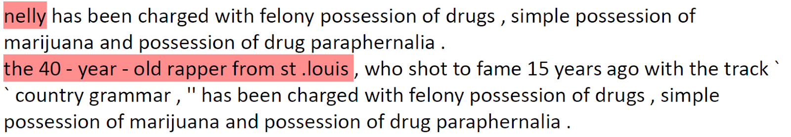
As you can see, the noun nelly is used before the pronoun the 40-year-old rapper from st. louis is used and fixes the problem of pronouns being used before being defined. 

However, this model has two problems: there's no rule that's taken into consideration when putting the pronouns back during post-processing and this model uses more time and space while running. While the dictionary that is saved locally contains the right pronouns, each of the pronouns differ in context and meaning. For example, his and him are both pronouns but are used in different contexts. But because we have no idea how the baseline model is going to produce a summary, we have no idea which pronouns to save locally and which pronoun to add back into the generated summary to make sure the correct pronoun is used. There also has not been enough research done in coreference resolution field where a machine can learn to put which pronoun into where. So this model currently puts pronouns in consecutive order from the dictionary but may put in wrong pronouns at times.

In addition, because the model has to pre-process and post-process each data, this adds computation time (even when the process is done through multiple threads) and uses space to save the information from pre-processing to be used later. Because of these two increase in costs, I came up with a third way in tackling the pronoun ambiguity problem.

Coreference Resolution Pipeline

Instead of processing the data, I wanted a way for the model to learn to mention the noun before producing a pronoun. This led to the creation of the following model:

Simply put, I add a third pipeline of data that is for pronouns. If you can recall from the baseline model section above, there are two existing pipelines of data: one from the source text (attention distribution) and one from the vocabulary pool (vocabulary distribution). I add a third pipeline that is trained purely on just the nouns that have pronouns in the reference summary (e.g. "Wayne saw himself." becomes [84123, 1512, 634] as per the process of changing words into their IDs which then gets processed and becomes [84123, 0, 0]). By doing so, I add more weight into the words that are nouns with pronouns. This pipeline of data is then taken into consideration at the final step of the baseline model where the switch lies. After the switch determines to take the data from either the attention distribution or the vocabulary distribution, the goes to another switch where it detects if the word that is to be generated is a pronoun or not. If it is a pronoun, it then refers to the third pipeline of data where heavy emphasis has been put into the noun that the pronoun is referring to. It then considers both the pronoun and noun and outputs whichever word has more probability (the noun in most cases). This model aims to mainly solve the problem of pronouns being used without being defined first which creates the most confusion in a generated summary compared to the other pronoun issues.

Here is a summary generated by this model:

Pronoun ambiguity problem is also solved here as done in two_models. But this summary is definitely a lot cleaner and concise. This can be factored to the fact that this model considers data from the third pipeline which does not contain any information other than for the nouns. This gets rid of a lot of unneeded information from being processed and thus creates a more concise summary.

Experiment

The models are trained on ~300k CNN/Daily Mail news articles where each article is paired with reference summaries averaging about 3.75 sentences. A small vocabulary pool of size 50k was used compared to other top-of-the-line models out there that uses 150k vocabs. This is due to the baseline model's ability to handle OOV vocabulary words with pointers. 256-dimensional hidden states and 128-dimensional word embeddings are used as per the experiment done in the baseline model's experiment. Actually, almost everything was kept the same except for two things: max_enc_steps and max_dec_steps. These two parameters determine the maximum number of source text tokens and summary tokens to look at while encoding and decoding respectively. While the baseline experiment uses 400 tokens for encoding and 100 tokens for decoding, I had to use 300 tokens and 75 tokens to account for my system's computational limits (my GTX 1080 GPU compared to baseline's Tesla K40m GPU). The baseline was trained for 4 days with each training step taking about 0.5 seconds, two_model was trained for 2 days with 0.7 seconds per step, and coreference_resolution_pipeline was trained for 1 day with 0.9 seconds per step.

ROUGE

Before we get into results, we need to cover a scoring package generally used to automatically evaluate generated summaries: Recall-Oriented Understudy for Gisting Evaluation (ROUGE). For our experiment, we use three specific categories of ROUGE scores: ROUGE-1, ROUGE-2, and ROUGE-L. ROUGE-1 measures the overlap of unigrams between the generated summary and the reference summary, ROUGE-2 measures the overlap of bigrams between the generated summary and the reference summary, and ROUGE-L measures the longest matching sequence of words using Longest Common Subsequence (LCS) based statistics. LCS is utilized because unlike substrings, subsequences are not required to occupy consecutive positions within the original sequences. This gives more room for abstract summaries to not get docked for creating summaries that do not resemble the reference summary too closely but still does a great job. Within each of these 3 categories, there are 3 scores: recall, precision, and f-score. Recall measures how much of the reference summary the generated summary is recovering/capturing, precision measures how much of the generated summary is relevant/needed, and f-score is a score that takes the harmonic average of the recall score and the precision score.

Results

(Higher is better)

From this chart, we can clearly see that both two_models and coreference_resolution_pipeline models excel the baseline model but a slight margin. The only category the baseline model does better in is the precision scores in all three of the unigram, bigram, and lcs categories. But it is clear that both models make improvements upon the baseline model. While these improvements may be small, it is important to note that the two newly created models was trained for a significantly less amount of time especially the coreference_resolution_pipeline model that was only trained for a day compared to the baseline model's training of 4 days. This gives the idea of how less amount of data can be used for a less amount of time in training a model to create a better summary.

Conclusion

While both of the solutions proposed and experimented in this project can be refined significantly in terms of optimization, the results tell us that a model that was trained on less amount of data (third pipeline) for a lot shorter period of time can do as well as if not outperform models out there in terms of dealing with pronouns and creating a more concise summary. As researches in both automatic abstract text summarization and coreference resolution field continue, hopefully there may be a day for a general tool to be developed in summarizing not only new articles but also academic papers, textbooks, and much more to speed up the time in learning new materials.